Building a RAG Pipeline over 17,000 PDFs
A build log for a RAG system over thousands of real drug leaflets — PDF-to-markdown, section-aware chunking, a cross-encoder reranker, and GPU-scaled embeddings. The bugs that nearly sank it, with the numbers.
Most RAG tutorials start with a clean folder of .txt files. Real data starts with 25,000 PDFs behind a government API, half of them with a scanned page in the middle, all of them wrapped in the same legal boilerplate. The model you pick at the end matters far less than what you do to that text on the way in.
This is the build log for a RAG pipeline over the Italian drug leaflets — the Foglietti Illustrativi (FI) and Riassunti delle Caratteristiche del Prodotto (RCP) published by AIFA. It’s the applied companion to my privacy-first local RAG pillar: same shape, but at a scale where the plumbing decides everything. My one claim: on real documents, extraction + section-aware chunking + a reranker move answer quality more than swapping the LLM ever will. I spent ~10× the effort there, and it paid back ~10×.
The setup: a messy pharmaceutical dataset
The starting point was three CSVs from AIFA’s public medicines data, joined by shared drug/package codes.
atc.csv — 7,209 rows. The ATC (Anatomical Therapeutic Chemical) classification.
| Column | Meaning |
|---|---|
CODICE_ATC | ATC classification code |
DESCRIZIONE | Therapeutic category |
PA_confezioni.csv — 337,550 rows. Active ingredients per package.
| Column | Meaning |
|---|---|
CODICE_AIC | Marketing-authorization (AIC) code |
PRINCIPIO_ATTIVO | Active ingredient |
QUANTITA | Amount |
confezioni_fornitura.csv — 159,708 rows. The package registry, with the PDF links.
| Column | Meaning |
|---|---|
COD_FARMACO | Drug ID — identifies the two PDFs |
DENOMINAZIONE | Trade name |
RAGIONE_SOCIALE | Manufacturer |
CODICE_ATC | ATC code (→ atc.csv) |
CODICE_AIC | AIC code (→ PA_confezioni.csv) |
LINK_FI / LINK_RCP | PDF links: leaflet / SPC |
The join keys are clean: CODICE_ATC links the registry to the ATC table (100% match), CODICE_AIC links it to active ingredients, and COD_FARMACO identifies the two documents — the Foglietto Illustrativo (patient leaflet) and the Riassunto delle Caratteristiche del Prodotto (summary of product characteristics), reached through LINK_FI and LINK_RCP on AIFA’s API.
First useful observation: 159,708 rows, but only 12,599 unique drugs (COD_FARMACO). The FI/RCP links are per-drug, so deduplicating dropped the download from ~320,000 requests to 25,198 PDFs (one FI + one RCP each). A SELECT DISTINCT before you write the crawler is the cheapest optimization you’ll ever make.
The messy part is what’s missing: of the 25,198 links, ~7,000 return a 404 — drugs that were withdrawn or never had a leaflet published. That’s ~28% of the catalog with no document, and pretending otherwise would poison the corpus. Every miss goes into a missing.csv with the drug name, ATC code, and reason, so the gaps are auditable instead of silent.
The architecture is deliberately hybrid, not RAG-for-everything:
CSV (structured) ──► SQLite ──────────────────┐
                                              ├─► retrieve: SQL filter → vector search → rerank → LLM
PDFs ─► markdown ─► chunk ─► embed ─► ChromaDB┘
Tabular questions (“which company makes X”, “what’s the ATC code”) are exact lookups — that’s SQL, deterministic, zero hallucination. RAG is only for the free text of the leaflets: indications, dosage, contraindications, side effects. Forcing structured data through embeddings is a common and expensive mistake.
Step 1 — Getting to clean text
The leaflets are born-digital PDFs, so the text is really in there — no OCR needed for the body. pymupdf4llm turns each PDF into Markdown while keeping some structure:
import pymupdf4llm

md = pymupdf4llm.to_markdown(pdf_path, show_progress=False)
Two things bit me here, and both are in the numbers section below: a self-inflicted OCR slowdown, and the fact that “has structure” is not the same as “has usable headings.”
Step 2 — Chunking by section (the highest-leverage step)
RCP and FI documents have a standard section layout — RCP 4.1 Indications, 4.2 Posology, 4.3 Contraindications, 4.8 Undesirable effects, and so on. If you chunk on those boundaries, a query about side effects lands squarely in section 4.8. If you chunk blindly every N characters, you shred it.
The catch: pymupdf4llm doesn’t emit those as Markdown headings. It renders them as inline bold markers (**4.3 Controindicazioni**) sitting inside paragraphs. My first splitter keyed off # headings and produced garbage “sections” like page footers. The fix was to segment on the numbered bold markers wherever they appear:
import re

# matches "**4.3 Controindicazioni**" or "## 6.1 Eccipienti" anywhere in the text
SEC = re.compile(
    r"(?:\*\*|#{1,6}\s*)\s*(\d+(?:\.\d+)*)\.?\s+([A-ZÀ-Ù][^*\n]{2,90}?)\s*(?:\*\*|$)",
    re.M,
)
Two more cleanups earned their keep. Every document carries the same AIFA legal footer (“Documento reso disponibile da AIFA…”, “Esula dalla competenza dell’AIFA…”) — pure noise, repeated ~2,800 times across the pilot, stripped with a couple of regexes (99% gone). And I embed each chunk with its context baked in rather than raw text:
embed_text = f"{drug_name} — {doc_type} — {section}: {chunk}"
# stored document = raw chunk; the string above is what gets embedded
That prefix means the vector itself knows which drug and which section it came from — retrieval on a drug name or a section topic gets noticeably sharper.
Step 3 — Embeddings and the reranker that mattered
Embeddings use BAAI/bge-m3 — multilingual, long-context, strong on Italian medical text — kept at fp32 for maximum fidelity. Vectors go into ChromaDB on local disk.
The single change that moved quality most was two-stage retrieval: cast a wide net with dense search, then reorder with a cross-encoder.
# stage 1: dense recall
cands = collection.query(query_embeddings=[q_vec], n_results=30)

# stage 2: cross-encoder precision
scores = reranker.predict([(question, c) for c in cands["documents"][0]])
top = [c for _, c in sorted(zip(scores, cands["documents"][0]), reverse=True)][:6]
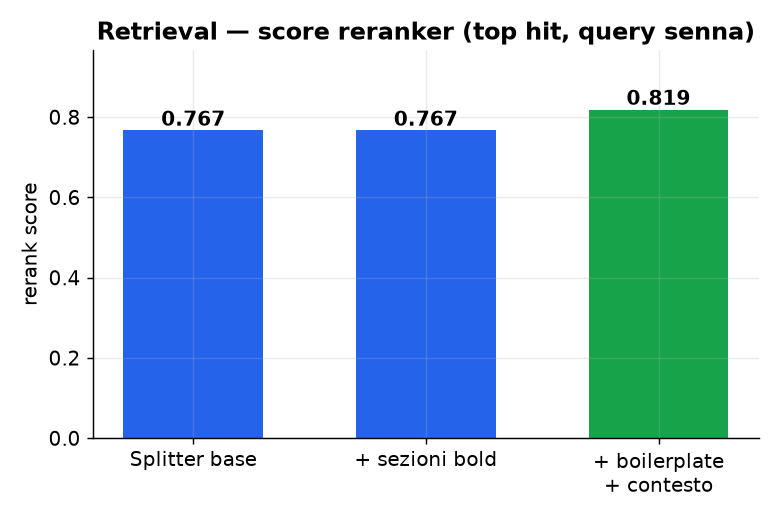
Dense search is fast but fuzzy; the bge-reranker-v2-m3 cross-encoder reads the question and each candidate together, so it ranks on actual relevance, not just cosine proximity. On a validation query (“contraindications and side effects of senna”) the top-hit rerank score went from 0.767 to 0.819 once section chunking, boilerplate stripping, and the context prefix were in place — and, more importantly, the top result became the actual 4.8 Undesirable effects section instead of a page header.
Where it broke
The interesting part. Four things nearly sank the run.
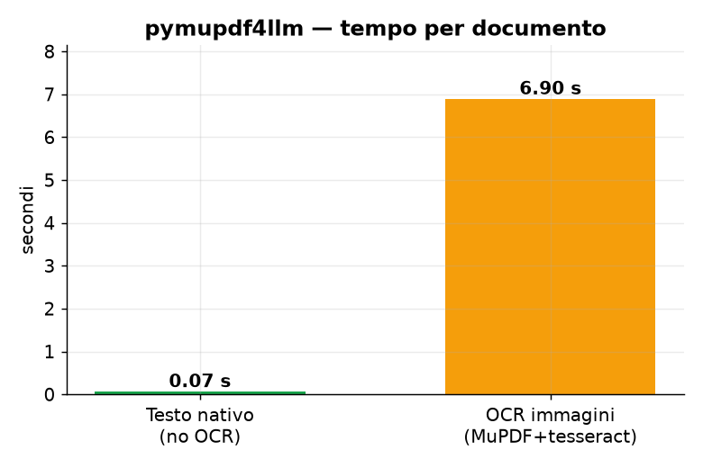
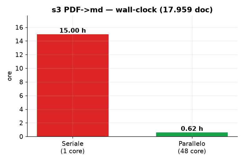
1. pymupdf4llm quietly OCR’d every image — 15 hours instead of 40 minutes. Locally the conversion flew; on the cloud box each document took ~7s. The difference: I’d installed tesseract for a separate step, and MuPDF, finding it, started OCR-ing every logo and watermark image in every PDF. Neither the library flags nor TESSDATA_PREFIX disabled it.
I stopped fighting it and parallelized instead — the box had 48 idle cores while a single one did all the parsing:
from multiprocessing import Pool
with Pool(48) as pool:
    for result in pool.imap_unordered(convert_one, todo, chunksize=8):
        ...
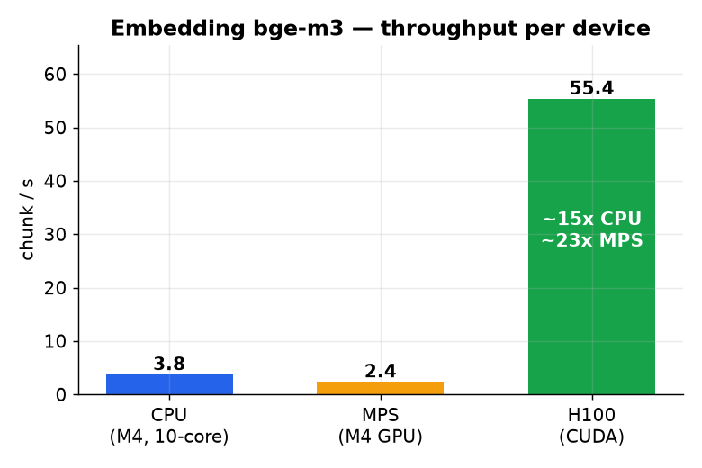
2. The GPU was slower than the CPU. On the Apple Silicon dev machine, embedding on MPS ran at ~2.4 chunks/s versus ~3.8 on the CPU — the integrated GPU plus operator fallbacks made it a net loss for a model this size. Don’t assume “GPU” means “faster”; measure.
3. torch’s CUDA didn’t match the driver. pip install torch pulled a CUDA 13 wheel onto a box with a CUDA 12.6 driver, so torch.cuda.is_available() was silently False. Installing the cu124 wheel fixed it. On Linux the wheel ships the CUDA runtime — you only need a compatible driver.
4. A full disk killed ChromaDB mid-write. The instance had a 40 GB root disk; the OS, the torch install, and the model cache ate ~26 GB before the ~11 GB index had anywhere to go. ChromaDB died with Error in compaction: Failed to apply logs to the metadata segment — which is just “disk full” in a trench coat. Mounting a separate volume and moving the data + model cache onto it fixed it.
The numbers
Embedding throughput, bge-m3, 256-chunk batches, across the three machines I actually ran it on:
| Device | chunks / s | Note |
|---|---|---|
| CPU (Apple M4, 10-core) | 3.8 | fine for a pilot |
| MPS (M4 GPU) | 2.4 | slower than the CPU |
| H100 (CUDA) | 55.4 | ~15× the CPU |
The full corpus came to ~805,000 chunks from ~17,959 converted documents (the ~7,000 missing were genuine 404s — drugs with no published leaflet, all logged to a missing.csv). Embedding that on the H100 took ~2.5 hours; on the CPU it would have been ~2 days.
What I’d actually keep
If I had to cut this pipeline to the parts that earned their complexity: section-aware chunking, the boilerplate strip, and the reranker. Those three are ~80% of the retrieval quality. The embedding model and the LLM are close to interchangeable by comparison — I’d happily run a smaller model with this retrieval stack over a frontier model with naive chunking.
The rest is discipline, not cleverness: dedup before you crawl, keep structured data in SQL, log what you couldn’t fetch, and measure the hardware instead of trusting the label on it. None of it is glamorous. All of it is what made the answers trustworthy.
If you build things like this, I write up more of them under RAG and AI × Backend — and the local-first version of the same ideas lives in the privacy-first local RAG guide and in Cosmind. More of the same on GitHub.
References
Related
A practical, end-to-end guide to building a private RAG system that never leaves your machine — local embeddings, vector store, and LLM, with real code.
How I wired Ollama into a real ASP.NET Core app with native tool-calling and a hand-rolled cosine-similarity RAG — no vector DB, no cloud API — and the concurrency bug that nearly broke it.
How I predicted California house prices with linear regression trained by gradient descent (SGDRegressor) — mutual-information feature selection, a scaling gotcha that breaks SGD, and an honest benchmark against KNN, a decision tree, and WEKA.
Get new posts by email
No hype, unsubscribe anytime. · Powered by Buttondown