I Built a House-Price Regressor: Linear Regression with Gradient Descent, scikit-learn vs WEKA
How I predicted California house prices with linear regression trained by gradient descent (SGDRegressor) — mutual-information feature selection, a scaling gotcha that breaks SGD, and an honest benchmark against KNN, a decision tree, and WEKA.
My linear regression series built the theory of fitting a line with gradient descent — the cost function, the gradients, feature scaling, R². This post puts it to work on real data, and is the regression companion to the speech-emotion classifier I wrote up earlier. The task: predict California house prices with linear regression trained by gradient descent, then ask the same question as before — does my scikit-learn pipeline agree with WEKA, and how much does insisting on a linear model cost me?
The code is in the repository. Here are the decisions, the scaling bug that nearly sank it, and the honest result.
The problem and the data
The California Housing dataset is 20,640 districts from the 1990 US Census, each with 8 numeric features — median income, house age, average rooms, population, location — and a target: the median house value of the district, in units of $100,000.
| Feature | What it measures |
|---|---|
| MedInc | Median income in the district |
| HouseAge | Median house age |
| AveRooms / AveBedrms | Average rooms / bedrooms per household |
| Population / AveOccup | District population / average occupancy |
| Latitude / Longitude | Where the district is |
No missing values, no duplicates — but one trap. The target is right-censored at 5.0 ($500k): every district worth more was clipped to exactly 5.0, producing a spike at the ceiling.
sns.histplot(data['MedHouseVal'], bins=50, color='#818cf8')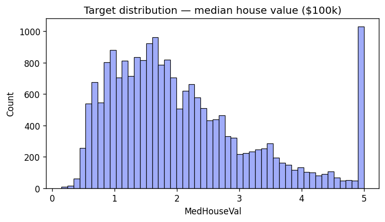
That spike matters: no model can predict values it never sees, so the cap puts a hard ceiling on accuracy. I kept those rows (the standard use of this dataset) but they explain a lot of the error later.
Feature engineering: keep what informs the target
I scored every feature by mutual information against the target — on the training set only, to avoid leaking test information — and kept those above 0.05.
mi = mutual_info_regression(X_train, y_train)
selected = ft_import[ft_import['Importance'] > 0.05].index.tolist()
# -> ['Longitude', 'MedInc', 'Latitude', 'AveRooms', 'AveOccup']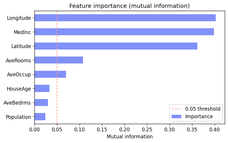
MedInc dominates (richer districts, pricier homes — no surprise), but the next strongest signals are Latitude and Longitude. That’s the first red flag for a linear model: price depends on where a district is in a deeply non-linear way (coastline, cities), and a straight-line fit can’t bend around a map.
The scaling bug that broke gradient descent
My first run with StandardScaler made the SGD loss explode to NaN. California has brutal outliers — a few districts with AveOccup in the thousands — and z-scoring leaves those as huge values that blow up the gradient. The fix: scale to [0, 1] with MinMaxScaler, which bounds every feature and keeps the steps stable. (It’s also what WEKA’s SGD does internally.)
pipe = Pipeline([('scaler', MinMaxScaler()),
                 ('regressor', SGDRegressor(loss='squared_error', max_iter=1000))])
Linear by gradient descent — and two non-linear baselines
The assignment’s pick for regression is linear regression with gradient descent, which is exactly SGDRegressor. To measure what linearity costs, I also ran a KNN regressor and a decision tree as non-linear baselines (these are different from the classifier’s chosen method, as the assignment’s point 5 requires). Three metrics on the 20% holdout:
- R² — fraction of target variance explained (1.0 is perfect, 0 is no better than the mean);
- MAE — mean absolute error, in $100k units;
- RMSE — root mean squared error, which punishes big misses harder.
| Model | R² | MAE | RMSE |
|---|---|---|---|
| Linear regression (SGD) | 0.526 | 0.580 | 0.786 |
| KNN | 0.786 | 0.349 | 0.528 |
| Decision Tree | 0.602 | 0.459 | 0.720 |
The linear model explains about half the variance — and the non-linear models beat it clearly. That gap is the finding, not a failure.
What the linear model can and can’t do
Plotting predicted against actual values shows exactly where it struggles:
plt.scatter(y_test, y_pred, s=4, alpha=0.2, color='#818cf8')
plt.plot([y.min(), y.max()], [y.min(), y.max()], 'r--')  # perfect-fit line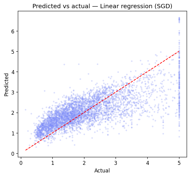
Two things jump out. The vertical stripe at 5.0 is the censored ceiling — the true value is clipped, so the model scatters its guesses up and down a wall it can’t cross. And the cloud fans out as prices rise: the model is confident and roughly right for cheap districts, but increasingly off for expensive ones. KNN (R² 0.79) does better precisely because it can capture the geographic, non-linear structure that MedInc alone misses. The linear model isn’t broken — it’s underfit by design, and seeing that is the point of fitting it.
scikit-learn vs WEKA
Same protocol in WEKA — 80/20 holdout, same selected features — and the now-familiar comparison:
comparison.plot(kind='bar') # R², MAE, RMSE — scikit-learn vs WEKA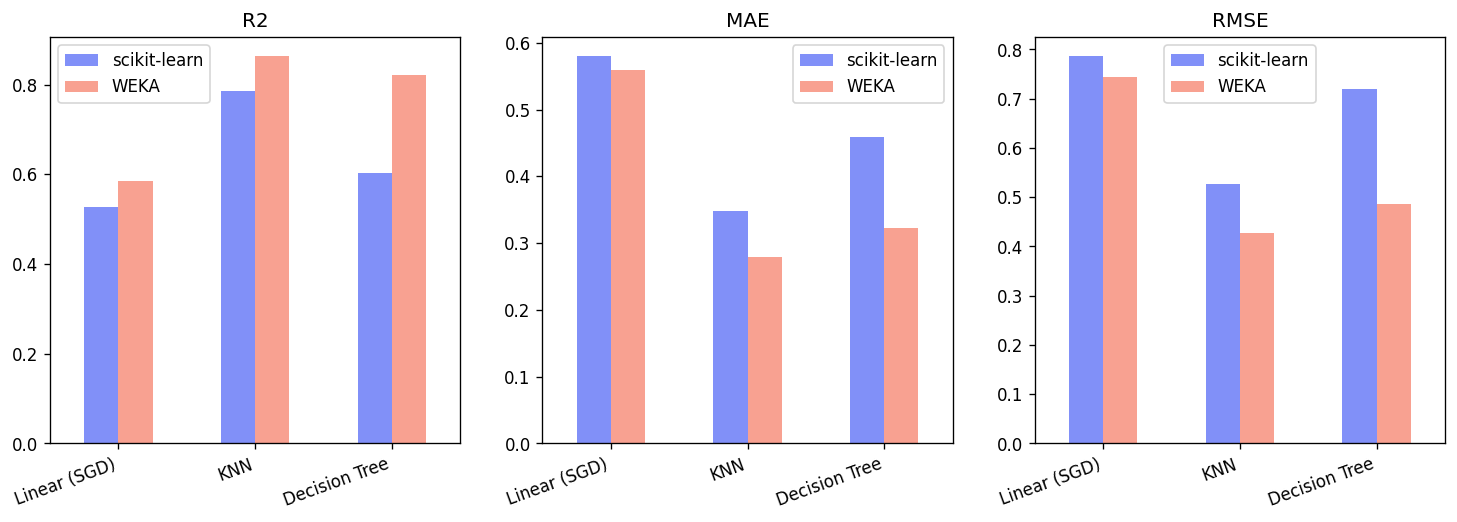
| Model | R² (sklearn / WEKA) | RMSE (sklearn / WEKA) |
|---|---|---|
| Linear regression | 0.526 / 0.586 | 0.786 / 0.745 |
| KNN | 0.786 / 0.863 | 0.528 / 0.428 |
| Decision Tree | 0.602 / 0.822 | 0.720 / 0.487 |
WEKA scored higher on every model, and the reasons mirror the classification post:
- Linear regression isn’t fit the same way. WEKA’s
LinearRegressionsolves the normal equations in closed form — the exact least-squares optimum. MySGDRegressorapproximates that optimum by gradient descent, which is the whole point of the assignment (“linear regression with gradient descent”). So WEKA edges ahead (0.586 vs 0.526), but it isn’t doing GD. - KNN and the tree diverge more, because WEKA’s defaults differ (neighbour count, tree pruning) — the same kind of implementation gap the classifier showed.
The takeaway holds across both projects: a single library looks internally consistent; a second one tells you whether your numbers are about the method or about one library’s defaults.
What I took away
- A linear baseline is honest, not weak. Its R² of 0.53 and that fanned-out scatter are a measurement: they quantify exactly how much of house prices is not linear in these features.
- Gradient descent is sensitive to scale. With raw outliers SGD diverged to
NaN; bounding features to[0, 1]fixed it. Closed-form solvers never have this problem — but they aren’t gradient descent. - Know your target. The censoring at $500k caps what any model can score; spotting it in the histogram explained the stripe before I ever trained a model.
This is the regression leg of a broader project — the classification write-up is already up, and unsupervised learning (clustering / PCA) is next. Code and WEKA scripts are in the repository; the maths behind the line lives in my linear regression series.
References
Related
How I built a speech emotion recognition model in Python — parsing MFCC voice features, pruning them with mutual information, and benchmarking five classifiers (logistic regression, naïve Bayes, KNN, decision tree, MLP) in scikit-learn against WEKA.
Predicting California house prices with linear regression trained by gradient descent — benchmarked against KNN, a decision tree, and WEKA.
What is multivariate (multiple) linear regression? Learn how this ML algorithm fits a hyperplane with one weight per feature plus a bias to predict values from many inputs.
Get new posts by email
No hype, unsubscribe anytime. · Powered by Buttondown