What Is Univariate Linear Regression? How It Works in ML

Linear regression is a statistical method used to model the relationship between variables. In ML (Machine Learning), it is used to predict a target value from one or more input features.

Let’s take the following graph of housing costs as an example:

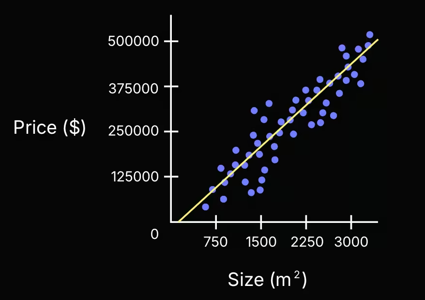
We can see the regression line passing through the data points.

Linear Regression Equation

The formula is simple and goes as follows: $y'=wx+b$ Where:

• $y'$: expected output, prediction;
• $w$: weight (the slope of the line);
• $x$: input, the feature value;
• $b$: model bias.

The $w$ and $b$ are both calculated during the training session.

Loss and Cost Function

To evaluate this model, we must distinguish between:

• loss function: computes the error for a single training example;
• cost function: overall error cost of the entire training set.

Loss Function

The loss function measures the error on a single training example.

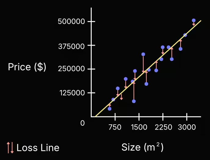
The two basic forms:

Where:

• $y_i$: the actual (observed) value of the $i$-th sample;
• $\hat{y}_i$: the value predicted by the model for the $i$-th sample.

Cost Function

The cost function aggregates the loss over the entire training set of $N$ samples.

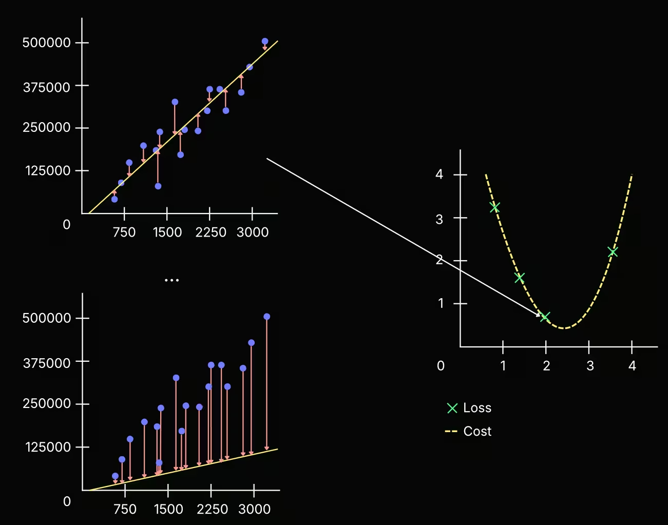
There are three main equations:

Where:

• $y_i$: the actual (observed) value of the $i$-th sample;
• $\hat{y}_i$: the value predicted by the model for the $i$-th sample;
• $N$: the total number of samples.

MAE is the mean of the $L_1$ loss, MSE the mean of the $L_2$ loss, and RMSE the square root of MSE.

The most used are MAE and RMSE because they are more human-interpretable: they keep the error on the same scale as the data, instead of inflating it like MSE or the $L_2$ loss.

Gradient Descent

It is an algorithm that iterates over the model’s weights and biases to find the model with the lowest cost. To better understand this, consider the following comparison: the cost function is used to calculate how much the model is off the mark based on all the loss functions; gradient descent, on the other hand, is the algorithm that optimizes the model by adjusting its parameters to minimize that cost.

The process works as follows:

1. Calculate the cost using the current weights and biases;
2. Determine in which direction to adjust (and consequently change) the weights and biases to reduce the cost;
3. Modify the weights and biases to actually reduce the cost;
4. Return to step 1 and repeat the process until the model reaches the desired low cost level.

repeat until convergence {
	grad_w = ∂J/∂w
	grad_b = ∂J/∂b

	w = w - α * grad_w
	b = b - α * grad_b
}

Where:

• $J$: cost function (the cost to be minimized);
• $\frac{\partial J}{\partial w}$, $\frac{\partial J}{\partial b}$: gradient indicates the direction of maximum cost growth, so we move in the opposite direction;
• $\alpha$: learning rate controls the step size at each iteration.

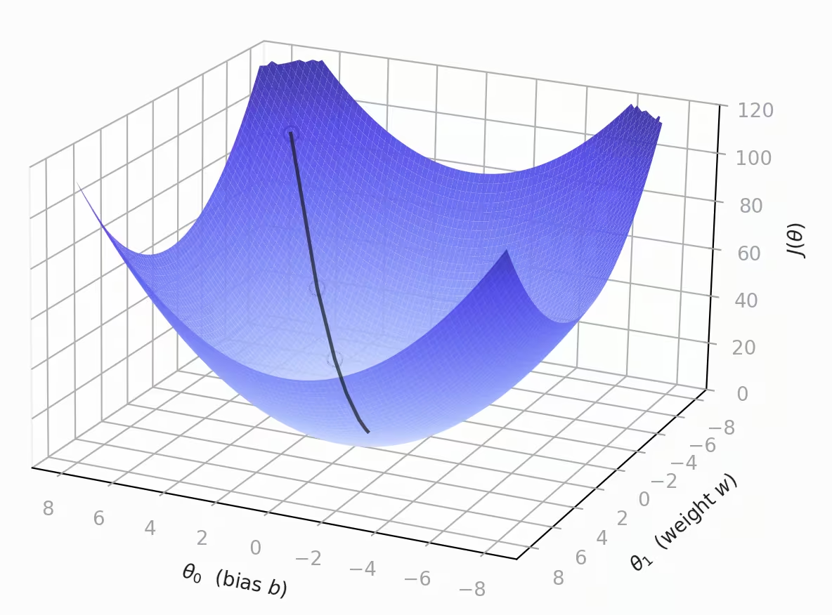
The parameters must be updated simultaneously: calculate both gradients using the old values of $w$ and $b$, then update them.

The above is the general form of gradient descent: it applies to any model, because the gradients remain symbolic. It becomes specific to linear regression when we expand those derivatives using the MSE cost function, $J = \frac{1}{N}\sum_{i=1}^{N}(\hat{y}_i - y_i)^2$, and the model $\hat{y}_i = w x_i + b$.

When we take the derivative, the exponent $2$ of the squared term comes down by the power rule and appears as a factor in the gradients. The cost function itself does not contain any $2$; it is produced by the derivative of the square.

$\frac{\partial J}{\partial w} = \frac{2}{N}\sum_{i=1}^{N}(\hat{y}_i - y_i)\,x_i \qquad \frac{\partial J}{\partial b} = \frac{2}{N}\sum_{i=1}^{N}(\hat{y}_i - y_i)$

Substituting into the update rule:

$w := w - \alpha \, \frac{2}{N}\sum_{i=1}^{N}(\hat{y}_i - y_i)\,x_i \qquad b := b - \alpha \, \frac{2}{N}\sum_{i=1}^{N}(\hat{y}_i - y_i)$

With the cost defined as $\frac{1}{N}\sum(\hat{y}_i - y_i)^2$, the factor $2$ remains in the gradients, exactly as stated above. Some, however, define the cost as $\frac{1}{2N}$: in that case, the $\frac{1}{2}$ and the $2$ in the derivative cancel out, and the gradients do not include the $2$. These are two equivalent conventions (in practice, the $2$ can still be absorbed into the learning rate $\alpha$).

Evaluating the Fit: R²

Loss and cost tell the optimizer how to improve the model, but they are in squared units and hard to read on their own: is an MSE of $12$ good? It depends entirely on the data. To judge how well the model actually fits, we use the coefficient of determination, $R^2$.

It measures the fraction of the variance in the target that the model explains, on a $0$-to-$1$ scale:

• $R^2 = 1$: the model predicts every point perfectly;
• $R^2 = 0$: the model does no better than always predicting the mean $\bar{y}$;
• $R^2 < 0$: it does worse than that trivial baseline.

$R^2 = 1 - \frac{\sum_{i=1}^{N}(y_i - \hat{y}_i)^2}{\sum_{i=1}^{N}(y_i - \bar{y})^2}$

The numerator is the squared error the model still makes; the denominator is the error of the trivial model that always predicts the mean. So $R^2$ is the share of that baseline error the model removes.

It is called the coefficient of determination because it is the square of the Pearson correlation coefficient $r$ between the observed values $y_i$ and the model’s predictions $\hat{y}_i$:

$r = \frac{\sum_{i=1}^{N}(y_i - \bar{y})(\hat{y}_i - \bar{\hat{y}})}{\sqrt{\sum_{i=1}^{N}(y_i - \bar{y})^2}\;\sqrt{\sum_{i=1}^{N}(\hat{y}_i - \bar{\hat{y}})^2}} \qquad R^2 = r^2$

Equivalently, $r = \dfrac{\operatorname{cov}(y, \hat{y})}{\sigma_y\,\sigma_{\hat{y}}}$: covariance of observed and predicted, normalized by their standard deviations.

With a single feature there is a nice shortcut: since the prediction $\hat{y} = wx + b$ is just a straight-line transform of $x$, the correlation between $y$ and $\hat{y}$ equals the correlation between $y$ and the feature $x$. So in univariate regression “how well the line fits” and “how correlated $x$ and $y$ are” are the same question and $R^2 = r_{xy}^2$. With more than one feature that shortcut breaks: only the observed-vs-predicted form survives.

Where this goes next

That last caveat is the whole reason for the next step: multivariate linear regression is this same machinery with one weight per feature, fitting a hyperplane instead of a line.

If you’d rather see the math run on real data than on a clean example, the house-price regressor I built trains exactly this with gradient descent on 20,640 California districts — including the scaling gotcha that sent the gradient to NaN. And when the target is a class rather than a number, the line gets squashed through a sigmoid: that’s logistic regression.