What Is Multivariate Linear Regression? How It Works in ML

We talked about univariate linear regression and saw that it can handle only one feature. Multivariate (or multiple) linear regression can handle many features at once.

Where univariate fits a line, multivariate fits a hyperplane: one weight per feature, plus a single shared bias.

Multivariate Linear Regression Equation

With $n$ features, the prediction becomes:

$y' = w_1x_1 + w_2x_2 + \cdots + w_nx_n + b$

Each feature $x_j$ gets its own weight $w_j$, and $b$ is the bias. In compact vector form:

$y' = \mathbf{w} \cdot \mathbf{x} + b = \sum_{j=1}^{n} w_j x_j + b$

Where:

• $\mathbf{x} = [x_1, x_2, \ldots, x_n]$: the feature vector;
• $\mathbf{w} = [w_1, w_2, \ldots, w_n]$: the weight vector (one weight per feature);
• $b$: the model bias.

Univariate is just the special case where $n = 1$, which collapses back to $y' = wx + b$.

Loss and Cost Function

The loss and cost functions do not change. They only compare a predicted value $\hat{y}_i$ to the actual value $y_i$, so they don’t care how many features produced that prediction. The MSE (most used for multivariate) cost is still:

$J = \frac{1}{N}\sum_{i=1}^{N}(\hat{y}_i - y_i)^2$

The same goes for R², the evaluation metric we covered in the univariate post: it still works here, but only in its general form, as the square of the Pearson correlation between the observed values and the predictions, not the shortcut between a single feature and the target.

Gradient Descent

The only difference is that now we have one partial derivative per weight, plus one for the bias. Each weight $w_j$ is updated using its own feature $x_j$:

$\frac{\partial J}{\partial w_j} = \frac{2}{N}\sum_{i=1}^{N}(\hat{y}_i - y_i)\,x_{ij} \qquad \frac{\partial J}{\partial b} = \frac{2}{N}\sum_{i=1}^{N}(\hat{y}_i - y_i)$

Where $x_{ij}$ is the value of feature $j$ in sample $i$.

As before, all parameters must be updated simultaneously, using the old values:

$w_j := w_j - \alpha\,\frac{\partial J}{\partial w_j} \qquad b := b - \alpha\,\frac{\partial J}{\partial b}$

In pseudocode, the only change from the univariate version is that we loop over the $n$ weights, computing every gradient before applying any update:

repeat until convergence {
	for j = 1 to n {
		grad_w[j] = ∂J/∂w[j]
	}
	
	grad_b = ∂J/∂b

	for j = 1 to n {
		w[j] = w[j] - α * grad_w[j]
	}
	b = b - α * grad_b
}

Feature Scaling

With univariate regression there is only one feature, so its scale is not a problem. With multiple features it becomes one: real datasets mix features on completely different ranges. Predicting a house price, the number of rooms might span $1$–$5$ while the surface area spans $500$–$5000$. The model treats those raw numbers as comparable when they are not.

This hurts gradient descent. A feature with a large range produces large gradients, so its weight wants big steps; a feature with a small range wants tiny ones. With a single learning rate $\alpha$ shared by all weights, you cannot satisfy both: the cost surface becomes a stretched, narrow valley, and the algorithm zig-zags slowly toward the minimum instead of heading straight for it.

For example, this is without scaling, and produces slower convergence:

$x_1=\text{size}(500-5000)\qquad x_2=\text{number of bedrooms}(1-5)$

This is with scaling and produces faster convergence:

$x_1=\frac{\text{size}}{5000}\qquad x_2=\frac{\text{number of bedrooms}}{5}$

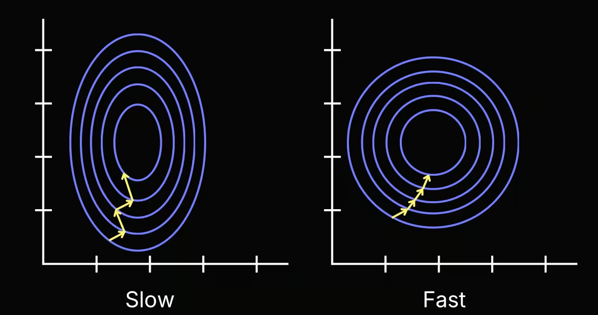
Feature scaling brings every feature onto a similar range, which makes the cost surface more symmetric and convergence faster and more stable.

There are two common methods:

Where:

• $\mu$: feature mean;
• $\sigma$: standard deviation.

Scale every feature before training, and apply the same transformation (the same $x_{\min}$, $x_{\max}$, $\mu$, $\sigma$ computed on the training set) to any new data at prediction time.

Choosing the Learning Rate

The learning rate $\alpha$ controls how big each step is during gradient descent, and it is the parameter you tune the most:

• too small: model converges, but very slowly, wasting many iterations.
• too large: steps overshoot the minimum; the cost oscillates or even grows, and the model can diverge.

The practical way to pick it is to plot the cost $J$ against the number of iterations (the learning curve) for a few values, for example $0.001$, $0.01$, $0.1$, $1$. A good $\alpha$ makes the cost decrease smoothly on every iteration. If the curve goes up or oscillates, $\alpha$ is too large; if it crawls down, it is too small.

This is also where feature scaling pays off: once all features share a similar range, a single $\alpha$ works well for every weight, so finding a good learning rate becomes much easier.

Features and Polynomial Regression

So far we have used features exactly as they come in the dataset, but we are free to build better ones. Predicting a house price from its frontage and depth, instead of feeding both as separate features you could multiply them into a single, more meaningful one, the area:

$x = \text{frontage} \times \text{depth}$

Choosing and transforming features like this, using what you know about the problem, is called feature engineering, and it often matters more than the model itself.

The same trick lets a linear model fit curves. When the data does not follow a straight line, you can add powers of a feature as new features. A cubic model of one feature $x$ is:

$y' = w_1 x + w_2 x^2 + w_3 x^3 + b$

If we set $x_1 = x$, $x_2 = x^2$ and $x_3 = x^3$, this is exactly the multivariate equation from before. The key point is that the model is still linear in the weights $w$, which is what “linear regression” really means, it does not have to be linear in $x$. Other transforms work the same way, for example a square root:

$y' = w_1 x + w_2 \sqrt{x} + b$

This is also where feature scaling becomes essential. If $x$ ranges from $1$ to $1000$, then $x^2$ ranges up to $10^6$ and $x^3$ up to $10^9$, so without scaling these derived features sit on wildly different ranges and gradient descent struggles.