What Is Logistic Regression? How It Works in ML

We covered univariate and multivariate linear regression, which predict a continuous number: a price, a temperature, a length. Logistic regression answers a different question: which class does this example belong to? It is a classification algorithm, not a regression one, despite the name.

The simplest case is binary classification: the target is one of two labels, encoded as $0$ or $1$ (spam / not spam, fraud / legit, churn / stay). Instead of predicting the label directly, logistic regression predicts the probability that the example belongs to the positive class, then turns that probability into a label.

Why Not Just Use Linear Regression?

A linear model $z = wx + b$ outputs any real number, from $-\infty$ to $+\infty$. A probability must live in $[0, 1]$. Feeding raw $z$ as a probability breaks immediately: a confident example could score $7.3$ or $-4$, which means nothing as a probability.

We need to squash that unbounded score into $[0, 1]$. That is exactly what the sigmoid (logistic) function does.

Sigmoid Function

The sigmoid maps any real number to the open interval $(0, 1)$:

$\sigma(z) = \frac{1}{1 + e^{-z}}$

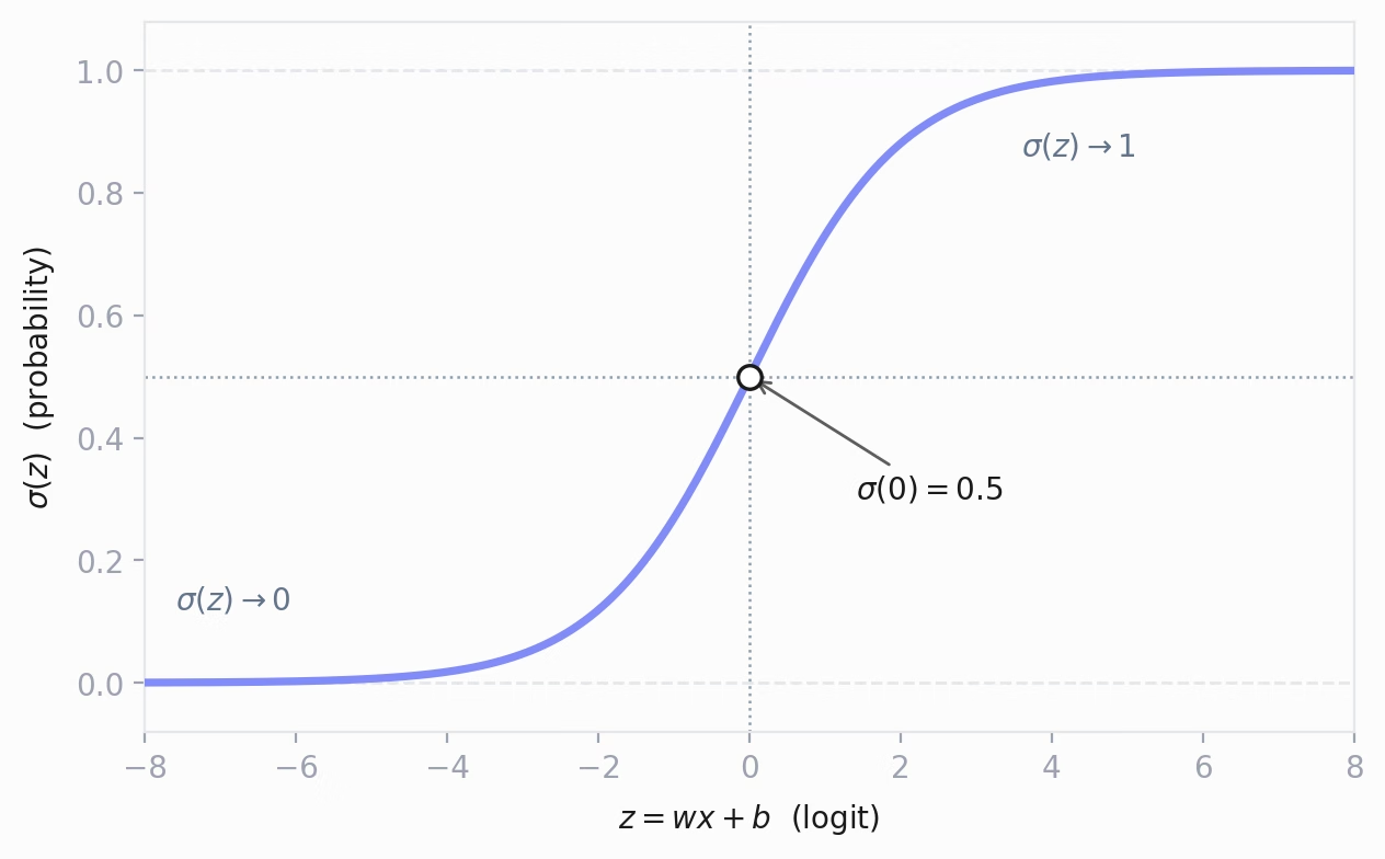
Its behavior is what we want from a probability:

• $z \to +\infty$: $\sigma(z) \to 1$;
• $z \to -\infty$: $\sigma(z) \to 0$;
• $z = 0$: $\sigma(z) = 0.5$ (the midpoint).

The curve is smooth and S-shaped: small near the extremes, steepest around $z = 0$. That steep middle is what lets a small change in the input flip the predicted class.

Logistic Regression Equation

Logistic regression is a linear model wrapped in a sigmoid. First it computes the same weighted sum as linear regression, the logit $z$:

$z = wx + b = \sum_{j=1}^{n} w_j x_j + b$

Then it passes $z$ through the sigmoid to get a probability:

$\hat{y} = \sigma(z) = \frac{1}{1 + e^{-(wx + b)}}$

Where:

• $x$: the feature vector;
• $w$: the weight vector (one weight per feature);
• $b$: the model bias;
• $\hat{y}$: the predicted probability that $y = 1$, i.e. $\hat{y} = P(y = 1 \mid x)$.

The linear part is identical to multivariate regression. The only new piece is the sigmoid on top, which is what converts a score into a probability.

Decision Boundary

A probability is not yet a label. To get a class, we compare $\hat{y}$ to a threshold, usually $0.5$:

• $\hat{y} \ge 0.5 \Rightarrow$ predict class $1$;
• $\hat{y} < 0.5 \Rightarrow$ predict class $0$.

Because $\sigma(z) = 0.5$ exactly when $z = 0$, the threshold on $\hat{y}$ is equivalent to a threshold on the logit:

$\hat{y} \ge 0.5 \iff z = wx + b \ge 0$

The set of points where $z = 0$ is the decision boundary. With two features it is a straight line; with $n$ features it is a hyperplane, splitting the feature space into the two predicted classes.

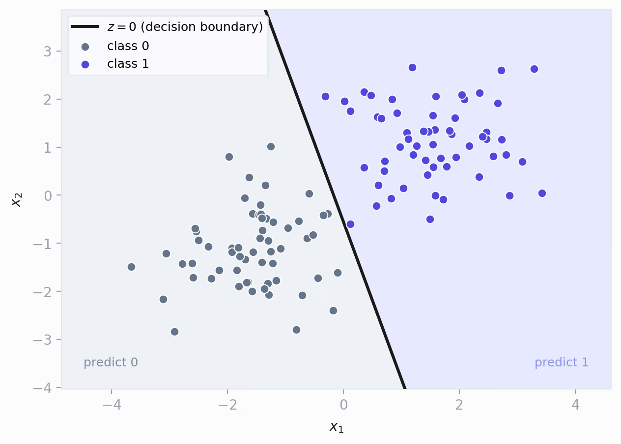
The boundary is linear in the features, even though the probability surface is curved by the sigmoid. The threshold does not have to be $0.5$: raise it to be more conservative about predicting the positive class (higher precision), lower it to catch more positives (higher recall). More on that below.

Loss and Cost Function

For linear regression we used MSE. For logistic regression MSE is a bad choice: paired with the sigmoid it produces a non-convex cost surface full of local minima, so gradient descent can get stuck. We need a loss that is convex for this model and that punishes confident wrong answers hard.

That loss is log loss, also called binary cross-entropy. For a single example:

$L = -\big[\,y\log(\hat{y}) + (1 - y)\log(1 - \hat{y})\,\big]$

Only one term is ever active, because $y$ is $0$ or $1$:

The logarithm is the key: a prediction that is both confident and wrong (say $\hat{y} = 0.01$ when $y = 1$) drives the loss toward infinity, so the model is strongly pushed to fix it.

The cost function averages this loss over all $N$ training examples:

$J = -\frac{1}{N}\sum_{i=1}^{N}\big[\,y_i\log(\hat{y}_i) + (1 - y_i)\log(1 - \hat{y}_i)\,\big]$

Where:

• $y_i$: the actual label ($0$ or $1$) of the $i$-th sample;
• $\hat{y}_i$: the predicted probability for the $i$-th sample;
• $N$: the total number of samples.

Gradient Descent

We minimize $J$ the same way as in linear regression: gradient descent. The remarkable part is that, after differentiating log loss through the sigmoid, the gradients come out in exactly the same form as the MSE gradients for linear regression:

$\frac{\partial J}{\partial w_j} = \frac{1}{N}\sum_{i=1}^{N}(\hat{y}_i - y_i)\,x_{ij} \qquad \frac{\partial J}{\partial b} = \frac{1}{N}\sum_{i=1}^{N}(\hat{y}_i - y_i)$

Where $x_{ij}$ is the value of feature $j$ in sample $i$. The only difference from linear regression is hidden inside $\hat{y}_i$: here it is $\sigma(\mathbf{w}\cdot\mathbf{x}_i + b)$ rather than the raw linear output. There is also no factor of $2$, because it comes from log loss, not the squared error.

The update rule is unchanged, and all parameters are updated simultaneously using the old values:

$w_j := w_j - \alpha\,\frac{\partial J}{\partial w_j} \qquad b := b - \alpha\,\frac{\partial J}{\partial b}$

repeat until convergence {
	for j = 1 to n {
		grad_w[j] = (1/N) * Σ (σ(w·x + b) - y) * x[j]
	}

	grad_b = (1/N) * Σ (σ(w·x + b) - y)

	for j = 1 to n {
		w[j] = w[j] - α * grad_w[j]
	}
	b = b - α * grad_b
}

Everything we learned for the regression series carries over: feature scaling still speeds up convergence, and the learning rate $\alpha$ is still the knob you tune the most.

Evaluating a Classifier

For regression we judged the fit with R². That metric makes no sense for classes, so classification has its own toolbox, built from the confusion matrix: the four ways a binary prediction can land.

From these four counts we derive the core metrics:

Accuracy alone is misleading on imbalanced data: if $99\%$ of examples are negative, a model that always predicts $0$ scores $99\%$ accuracy while catching zero positives. Precision and recall expose that. They also trade off against each other through the threshold: raising it lifts precision but lowers recall, and vice versa. F1 balances the two in a single number.

To judge the model across all thresholds at once, plot the ROC curve (true-positive rate vs false-positive rate) and report the AUC, the area under it. AUC ranges from $0.5$ (random guessing) to $1$ (perfect ranking), and unlike accuracy it does not depend on a single threshold choice.

Beyond Two Classes: Multiclass

Just as multivariate regression generalized univariate to many features, logistic regression generalizes from two classes to many. Logistic regression is binary by nature, so the common trick is to break a $K$-class problem into many binary problems and combine their answers. Two strategies do this:

• One-vs-All (OvA), also called one-vs-rest: train one binary classifier per class, each asking “this class vs everyone else”. To predict, run all $K$ classifiers and pick the class whose classifier returns the highest probability.
• One-vs-One (OvO): train one binary classifier per pair of classes, each asking “class $i$ vs class $j$” using only the data of those two. That is $\binom{K}{2} = \frac{K(K-1)}{2}$ classifiers. To predict, every classifier votes for one of its two classes, and the class with the most votes wins.

With $5$ classes, OvA trains $5$ classifiers, OvO trains $10$. OvO grows quadratically, so it builds more models, but each one sees only two classes worth of data, which helps when training cost grows fast with dataset size. Both collapse to plain binary logistic regression at $K = 2$: a single classifier either way.