I Built a Speech Emotion Classifier: 5 ML Algorithms, scikit-learn vs WEKA
How I built a speech emotion recognition model in Python — parsing MFCC voice features, pruning them with mutual information, and benchmarking five classifiers (logistic regression, naïve Bayes, KNN, decision tree, MLP) in scikit-learn against WEKA.
My regression series and the logistic regression post built up the theory of supervised learning one equation at a time. This post is the other half: a real project where I put that theory to work. The task — predict a speaker’s emotion from the acoustic signal of their voice — and the question I really wanted to answer: does my from-the-docs scikit-learn pipeline agree with a battle-tested tool like WEKA, or do they quietly disagree?
The full code (notebook + WEKA scripts) lives in the repository. Here I walk through the decisions, the results, and the one comparison that genuinely surprised me.
Problem and Data
The Acoustic Emotion Vocal Signature dataset is 10,000 voice samples, each labelled with one of 10 emotional states (Angry, Bored, Calm, Confused, Excited, Fearful, Happy, Neutral, Sad, Surprised). Crucially, the classes are balanced (roughly 1,000 samples each) which matters a lot later.
data['Mood'].value_counts().plot(kind='bar')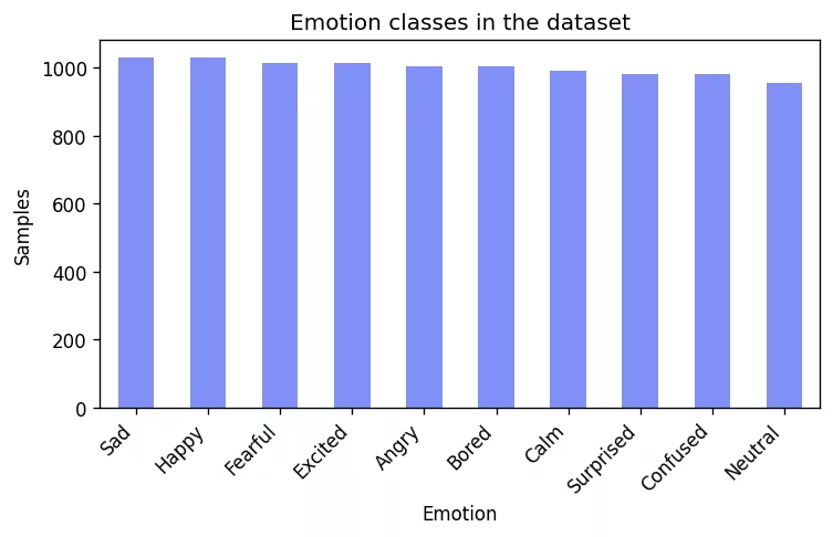
Each sample carries acoustic features:
| Feature | What it measures |
|---|---|
| Pitch | Voice frequency (Hz) |
| Speech Rate | Words per minute |
| Speech Duration | Length of the sample (s) |
| Jitter / Shimmer | Cycle-to-cycle variation in frequency / amplitude (%) |
| MFCCs | 13 coefficients describing the short-term power spectrum |
Plus metadata: gender, age group, language, a speaker ID and a sentiment score. Ten classes, mostly numeric features, no missing values, no duplicates. A clean starting point, but “clean” is not the same as “ready”.
Feature engineering: less is more
Three columns never made it to the model.
- Speaker ID and Language are noise: the ID is a random UUID, and every sample is English. Constant or unique columns teach a model nothing.
- Sentiment Score was dropped on purpose, and this is the interesting one. Sentiment is derived from the content of the speech, not its acoustic signal, and it correlates so tightly with the emotion label that it behaves like a near-leakage shortcut. The whole point of the project is recognising emotion from the acoustic signature; keeping sentiment would let the model cheat and quietly defeat the exercise.
The MFCCs column arrived as a string, like "[2.5, -0.06, -4.7, ...]". I parsed each one and exploded it into 13 numeric columns (MFCC_0 … MFCC_12), and encoded Gender and Age Group as integers, because scikit-learn models work with numbers, not raw category strings. That left 20 candidate features.
Picking features with mutual information
Twenty features, but how many actually carry signal about the emotion? I scored each one with mutual information; which, unlike linear correlation, also captures non-linear dependencies and is always ≥ 0 (0 means independent, higher means more informative).
The key discipline: compute it on the training set only. Touching the test set here would leak information about the very data you evaluate on later.
from sklearn.feature_selection import mutual_info_classif

importance = mutual_info_classif(X_train, y_train)
selected = importance[importance > 0.05].index.tolist()
# -> ['Pitch', 'Speech Rate', 'Speech Duration']ft_import.sort_values('Importance').plot(kind='barh')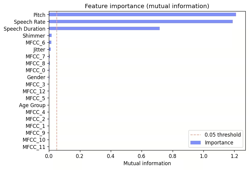
The verdict was blunt: only three features cleared the bar. Every MFCC coefficient, plus jitter and shimmer, scored ≈ 0 (pure noise for this dataset). And that noise isn’t harmless: irrelevant dimensions inflate distances and are exactly what drags down a distance-based model like KNN. Dropping 17 features wasn’t just tidy, it was a fix.
Five classifiers, one pipeline
The assignment let me pick one algorithm, but I implemented the whole shortlist so I could compare them honestly: logistic regression, naïve Bayes, KNN, a decision tree, and a single-hidden-layer MLP. (The theory behind logistic regression — sigmoid, log loss, the gradient that’s identical to linear regression’s, is in its own post.)
Every model ran inside the same pipeline, so preprocessing was identical and leak-free:
from imblearn.pipeline import Pipeline
from imblearn.under_sampling import RandomUnderSampler
from sklearn.preprocessing import StandardScaler

pipeline = Pipeline([
    ('undersampler', RandomUnderSampler(random_state=42)),
    ('scaler', StandardScaler()),
    ('classifier', model),
])
A stratified 80/20 holdout, then three metrics on the test set: accuracy, weighted F1, and weighted ROC AUC (one-vs-one). On a 10-class problem, random guessing scores 10% (so anything near 70% is doing real work).
| Model | Accuracy | F1 (weighted) | ROC AUC |
|---|---|---|---|
| Logistic Regression | 0.697 | 0.697 | 0.972 |
| Naïve Bayes | 0.709 | 0.710 | 0.973 |
| KNN | 0.684 | 0.684 | 0.954 |
| Decision Tree | 0.706 | 0.705 | 0.836 |
| MLP | 0.728 | 0.728 | 0.978 |
The MLP won on every metric. The decision tree’s accuracy is competitive, but its ROC AUC (0.836) is much lower; a single tree outputs crude, near-binary probabilities, so its ranking quality suffers even when its hard predictions are fine. ROC AUC is the metric I trust most here because it’s least sensitive to any residual imbalance and judges the model across all thresholds at once.
The confusion matrix shows where the best model slips — the off-diagonal cells are the emotions it mixes up (Bored↔Sad, Calm↔Neutral, Happy↔Excited):
sns.heatmap(confusion_matrix(y_test, mlp_pred),
			annot=True, fmt='d',
            cmap='Blues',
	        xticklabels=labels,
	        yticklabels=labels)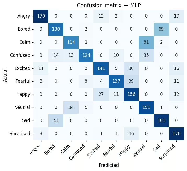
The real test: scikit-learn vs WEKA
A model is only as trustworthy as the validation behind it. So I reproduced the same protocol in WEKA (80/20 holdout, standardized features, the same three features) using FilteredClassifier so the scaler is fit on the training split only (no leakage), exactly like the scikit-learn pipeline. The algorithm mapping:
| scikit-learn | WEKA |
|---|---|
| LogisticRegression | functions.Logistic |
| GaussianNB | bayes.NaiveBayes |
| KNN | lazy.IBk -K 5 |
| DecisionTree (CART) | trees.J48 (C4.5) |
| MLP | functions.MultilayerPerceptron |
Side by side:
| Model | Accuracy (sklearn / WEKA) | ROC AUC (sklearn / WEKA) |
|---|---|---|
| Logistic Regression | 0.697 / 0.702 | 0.972 / 0.974 |
| Naïve Bayes | 0.709 / 0.715 | 0.973 / 0.975 |
| KNN | 0.684 / 0.817 | 0.954 / 0.989 |
| Decision Tree | 0.706 / 0.774 | 0.836 / 0.981 |
| MLP | 0.728 / 0.695 | 0.978 / 0.971 |
comparison.plot(kind='bar') # scikit-learn vs WEKA, one group per metric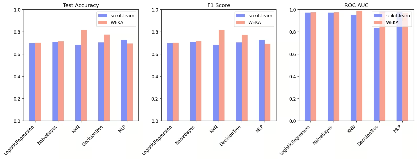
Logistic regression and naïve Bayes matched almost exactly; reassuring, since they’re the most standardized algorithms in both libraries. But KNN and the decision tree diverged hard, and that gap is the lesson of the project.
Two things explain it, and neither is a bug:
- The decision tree isn’t the same tree. WEKA’s
J48is C4.5; scikit-learn’s is CART. Different splitting criteria and pruning, so different results are expected; WEKA’s pruning also produces far better-calibrated probabilities, which is why its ROC AUC leaps from 0.836 to 0.981. - KNN exposes my preprocessing. The classes were already balanced, so the
RandomUnderSamplerin my pipeline buys nothing; it only throws away training data, and KNN is the model most sensitive to having fewer neighbours. WEKA, running plainIBkwith no resampling, kept all of it and scored 13 points higher. The honest takeaway: I added a step the data didn’t need, and the most fragile model paid for it.
That’s the value of cross-validating against a second tool. On its own, my notebook looked internally consistent. Against WEKA, it revealed a preprocessing choice I’d have otherwise never questioned.
What I took away
- Feature selection is a force multiplier. Cutting 20 features to 3 didn’t cost accuracy and made the distance-based models behave. More columns is not more signal.
- Guard against leakage on purpose, not by accident. Dropping sentiment score and fitting both the MI scorer and the scaler on training data only is what keeps the ~70% honest.
- Validate across tools, not just across folds. Two libraries agreeing builds confidence; two libraries disagreeing teaches you something — in my case, that an unnecessary resampling step was quietly hurting KNN.
This was the classification leg of a larger project that also covers regression and unsupervised learning — both writeups coming next. The code, the WEKA scripts, and the notebook are all in the repository; if you want the maths underneath the models, start with the logistic regression post.
References
Related
How I predicted California house prices with linear regression trained by gradient descent (SGDRegressor) — mutual-information feature selection, a scaling gotcha that breaks SGD, and an honest benchmark against KNN, a decision tree, and WEKA.
Predicting a speaker's emotion from the acoustic signature of their voice — five classifiers benchmarked in scikit-learn and cross-validated against WEKA.
What is logistic regression? Learn how this classification algorithm uses the sigmoid function, log loss, and gradient descent to predict probabilities and class labels.
Get new posts by email
No hype, unsubscribe anytime. · Powered by Buttondown